


Next: Implementation
Up: Self-organising maps of protein
Previous: Introduction
Contents
Self-organising maps - Overview
and Methods
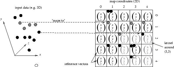
Kohonen's self-organising mapkohonen:som1,kohonen:som2 is an
unsupervised learning procedure based on a model of laterally interacting
neuronal units, resembling mechanisms proposed for stimulus recognition in
the cerebral cortex[Miller, 1994,Kohonen, 1993,Durbin & Mitchison, 1990]. In
broad overview, it projects high dimensional input data onto an ordered
two-dimensional grid, known as the map. As shown in Figure 5.1,
the map grid consists of reference vectors of the same dimensionality as
the input data. The mapping process is iterative, non-deterministic and
mathematically uncharacterised, but has the effect of preserving local
ordering relationships (as can be seen in the figure). There follows a
more rigorous explanation.
The map is a  array of reference vectors
  . At time
 , the map is initialised with random vectors within the ranges of the
input vectors. A total of
, the map is initialised with random vectors within the ranges of the
input vectors. A total of  training vectors
  are inputed to
Equations 5.1 and 5.2 at time points
are inputed to
Equations 5.1 and 5.2 at time points ![$t=[0..T]$](img238.gif) (input vectors repeated as necessary):
(input vectors repeated as necessary):
 |
(9) |
![\begin{displaymath}
r_{m,n}(t+1) = r_{m,n}(t) + k(m,n,r_w,d,t)\,a[1 - t/T]\,[v_i - r_{m,n}(t)]
\;\forall m,n
\end{displaymath}](img240.gif) |
(10) |
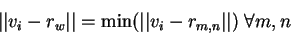
where  is the `winning' reference vector, the closest
reference vector to the input vector using the Euclidean distance metric.
The winning reference vector and its neighbours defined by the
neighbourhood kernel function
is the `winning' reference vector, the closest
reference vector to the input vector using the Euclidean distance metric.
The winning reference vector and its neighbours defined by the
neighbourhood kernel function
 are updated towards the
input vector (Equation 5.2). The kernel function basically
defines a set of neighbouring cells (shown in grey in
Figure 5.1). The kernel radius and learning rate, initially set
to
are updated towards the
input vector (Equation 5.2). The kernel function basically
defines a set of neighbouring cells (shown in grey in
Figure 5.1). The kernel radius and learning rate, initially set
to  and
and  respectively, decrease linearly with time to zero at the end
of the mapping procedure. At the end of the learning phase the training
vectors (or any other vector of the same dimension) can be mapped to a
winning vector on the output grid using Equation 5.1.
respectively, decrease linearly with time to zero at the end
of the mapping procedure. At the end of the learning phase the training
vectors (or any other vector of the same dimension) can be mapped to a
winning vector on the output grid using Equation 5.1.
Figure 5.1:
Some basic principles and definitions for
the Kohonen self-organising map.
 |
Subsections
Next: Implementation
Up: Self-organising maps of protein
Previous: Introduction
Contents
Copyright Bob MacCallum
- DISCLAIMER: this was written in 1997 and may contain out-of-date information.