advertisement: compare things at compare-stuff.com!

The dynamic programming alignment algorithm

The first application of dynamic programming to biological sequence alignment (both DNA and protein) was by Needleman and Wunschneedleman:wunsch. This and related algorithms have been in use since then for the detection of similarities (see Section 1.4.1) and the alignment of sequence information from protein families.

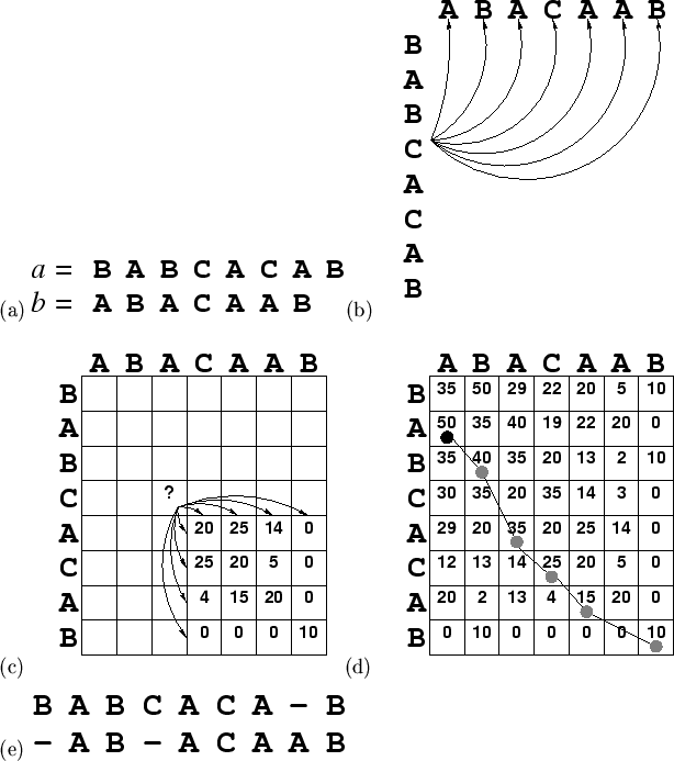
Figure 1.1(a) shows two short (imaginary) sequences we wish to align: sequence $a$ = BABCACAB, sequence $b$ = BCCAAB. Residues $i$ and $j$ in sequences $a$ and $b$ are denoted by $a_i$ and $b_j$ respectively. Similarly their lengths are denoted $m$ and $n$. The objective of any alignment algorithm is to maximise the alignment of similar or identical residues in $a$ with $b$, equivalent to $\sum{S_{i,j}}$ along the path of the alignment. $S_{i,j}$ is best explained as how `happy' residue $a_i$ is aligned against $b_j$.

Figure 1.1: The dynamic programming algorithm. (a) Unaligned sequences $a$ and $b$. (b) Pairwise suitability calculations. (c) Filling in the score matrix. (d) Complete score matrix and alignment trace-back. (e) Alignments between $a$ and $b$. Scoring with identity matrix (identity=10, otherwise=0), gap open penalty = 5 and gap extension penalty = 1. See text for full explanation.

In sequence comparison, the value of $S_{i,j}$ is looked up in a matrix $M$ containing the log-likelihoods of all substitutions between each of the 20 amino acids ( $20 \times 20 = 400$). $M$ is approximated from the frequencies of substitutions observed in sequence alignments[Barker & Dayhoff, 1972,Dayhoff et al., 1978,Henikoff & Henikoff, 1992]. Thus $S_{i,j}=M_{a_i,b_j}$ and when $a_i=b_j$, $M_{a_i,b_j}$ gives a high positive value. Smaller or negative values of $M_{a_i,b_j}$ occur when the amino acids $a_i$ and $b_j$ are less alike in terms of observed substitutions.

Gapless alignment of sequence $a$ and $b$ would simply involve sliding one sequence along the other and outputting the alignment where $\sum{S_{i,j}}$ is maximal, involving a number calculations only linearly dependent upon the sequence lengths. The allowance of gaps requires that each $a_i$ must be `tested' against $b_j$. Figure 1.1(b) illustrates the number of possibilities which exist in the alignment of residue $a_3$ (C) with sequence $b$. There are $m \times n$ such comparisons in total. Thus gapped alignments involve calculations scaling approximately to the square of number of residues.

The dynamic programming algorithm finds the optimal alignment through the construction of the $m \times n$ matrix $D$. The values of $D_{i,j}$ are filled in dynamically starting from the bottom right-hand corner as follows:

$$D_{i,j} = \max \left ( {\begin{array}{l} D_{i+1,j+1},\\ \\ ... ...m} (D_{i+1,j+q} - (g_o + g_e(q-j-2)))\\ \end{array}} \right )$$ (1)

where $g_o$ and $g_e$ are fixed penalties for the creation and extension of gaps, respectively. Figure 1.1(c) shows the matrix $D$ in the example partially filled in, and the scores from which $D_{3,2}$ are inherited. In this example the $M$ is the simple identity matrix (scoring 10 for identity and 0 otherwise); $g_o=5$ and $g_e=1$.

When complete, the highest value from the top and left edges of the matrix $D$ is found (marked with a black filled circle in Figure 1.1(d)) and the path which resulted in this score is traced back in reverse to generate the alignment, shown in Figure 1.1(e). A relatively minor modification to this algorithm was developed by Smith and Waterman[Smith & Waterman, 1981] to locate the best local alignments between two sequences. Local alignments are not required to include the termini of either sequence, as in the Needleman and Wunschneedleman:wunsch method which is a global alignment.