 |
(15) |
| advertisement: compare things at compare-stuff.com! |
In order to introduce information about hydrophobicity into the mapping
procedure we simply input four dimensional vectors as follows:
 |
(15) |
The vector, ![]() , has mixed units: Ångstrøms for the coordinates and
usually kcal/mol for the hydropathy (for the free energy of transfer from
an apolar solvent to a polar solvent, i.e. from octanol to water). This
immediately raises the problem of what weight to apply to the hydropathy
component in order for the correct balance of information to be present.
We were not in favour of normalising each vector component by its mean and
standard deviation, because this would distort the three-dimensional
coordinates. Instead we tested different weight factors,
, has mixed units: Ångstrøms for the coordinates and
usually kcal/mol for the hydropathy (for the free energy of transfer from
an apolar solvent to a polar solvent, i.e. from octanol to water). This
immediately raises the problem of what weight to apply to the hydropathy
component in order for the correct balance of information to be present.
We were not in favour of normalising each vector component by its mean and
standard deviation, because this would distort the three-dimensional
coordinates. Instead we tested different weight factors,
![]() , for the hydropathy component empirically as described
below.
, for the hydropathy component empirically as described
below.
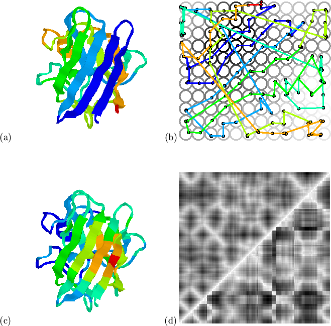
With
![]() the mapping, shown in
Figure 5.8, is broadly similar to that of structure
alone; structural constraints dominate and the mapping of hydropathy
preserves only its low-resolution features (see
Figure 5.8(c)), and loses the marked alternation in
the
the mapping, shown in
Figure 5.8, is broadly similar to that of structure
alone; structural constraints dominate and the mapping of hydropathy
preserves only its low-resolution features (see
Figure 5.8(c)), and loses the marked alternation in
the ![]() -sheet. The use of a larger hydropathy weighting
(
-sheet. The use of a larger hydropathy weighting
(
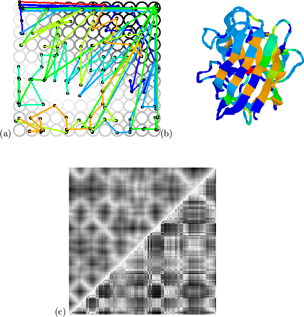
![]() ) creates a better balance between the two types
of information. The result, shown in Figure 5.9, is a
mapping which preserves the structural and hydrophobic relationships of
amphipathic sheet residues, whilst smoothing the hydrophobicity of loop
residues. The local relationships of residues which are close both in
space and hydrophobicity are retained by the mapping at the expense of
less well spatially correlated hydrophobics (in loop regions, for
example). As a result, more space in the map is devoted to these
points, and the map reference vectors more closely resemble the input
vectors for residues with `important' or spatially correlated
hydrophobicity. Conversely, isolated hydrophobic residues will map to
the same map vector as neighbouring less hydrophobic residues.
) creates a better balance between the two types
of information. The result, shown in Figure 5.9, is a
mapping which preserves the structural and hydrophobic relationships of
amphipathic sheet residues, whilst smoothing the hydrophobicity of loop
residues. The local relationships of residues which are close both in
space and hydrophobicity are retained by the mapping at the expense of
less well spatially correlated hydrophobics (in loop regions, for
example). As a result, more space in the map is devoted to these
points, and the map reference vectors more closely resemble the input
vectors for residues with `important' or spatially correlated
hydrophobicity. Conversely, isolated hydrophobic residues will map to
the same map vector as neighbouring less hydrophobic residues.
 |
 |
Other values for
![]() were tested and the simplest way to
visualise the results was a GIF (Graphics Interchange Format) animation.
The animation for domains 1sxaA0 and 1aak00[Cook et al., 1992] using values for
were tested and the simplest way to
visualise the results was a GIF (Graphics Interchange Format) animation.
The animation for domains 1sxaA0 and 1aak00[Cook et al., 1992] using values for
![]() are available on the
internet
are available on the
internet![]() .
The viewing of these animations is not essential. In summary, the highest
values of
.
The viewing of these animations is not essential. In summary, the highest
values of
![]() bias the mapping heavily towards the original
hydropathy data and look very much like Figure 5.7. As
bias the mapping heavily towards the original
hydropathy data and look very much like Figure 5.7. As
![]() decreases, the mapped hydropathy becomes more idealised
and the information in the loops decreases (as in
Figure 5.9) until a sudden change at
decreases, the mapped hydropathy becomes more idealised
and the information in the loops decreases (as in
Figure 5.9) until a sudden change at
![]() where the alternating patterns are lost (as in
Figure 5.8). The raw and mapped (
where the alternating patterns are lost (as in
Figure 5.8). The raw and mapped (
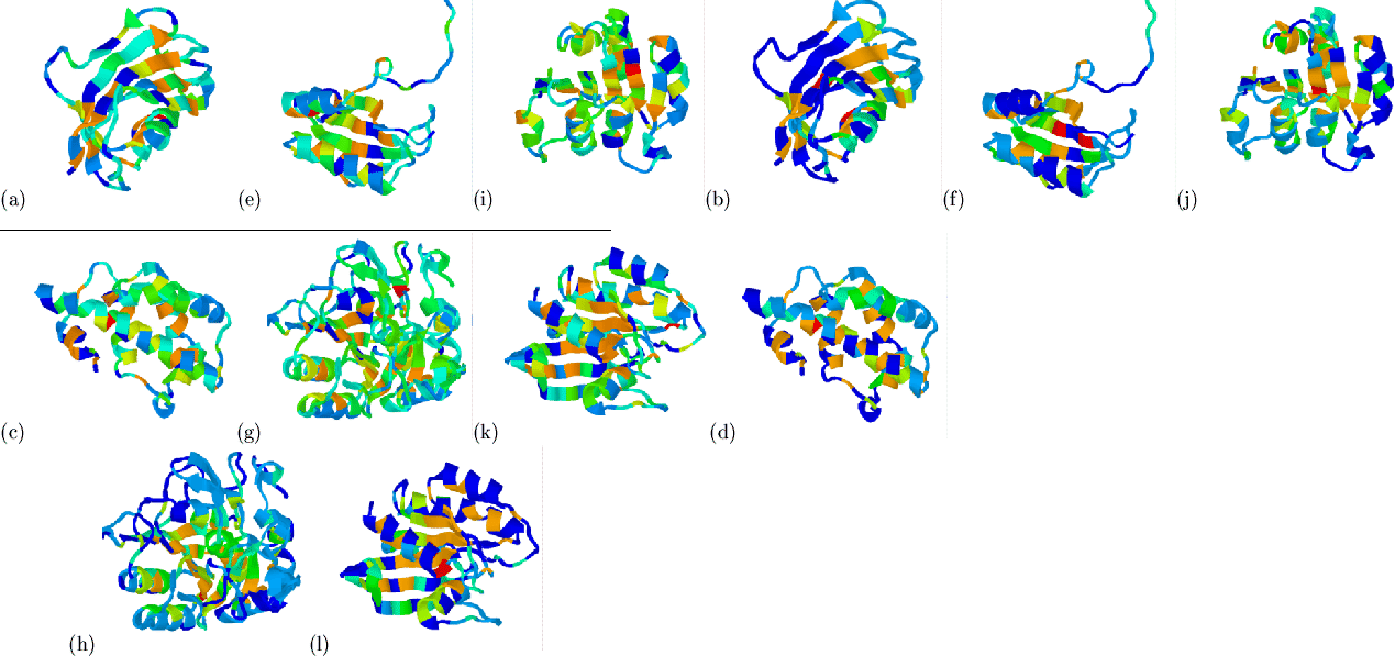
![]() )
hydrophobicities of a number of domains are shown in
Figure 5.10. The hydrophobic feature extraction appears
successful in each case (domains were picked at random from a list of 19
domains taken from CATH between 100 and 300 residues having at least 20
multiple sequences of not more than 70% pairwise identity). A
quantitative evaluation of these mappings is undertaken in
Section 5.5.
)
hydrophobicities of a number of domains are shown in
Figure 5.10. The hydrophobic feature extraction appears
successful in each case (domains were picked at random from a list of 19
domains taken from CATH between 100 and 300 residues having at least 20
multiple sequences of not more than 70% pairwise identity). A
quantitative evaluation of these mappings is undertaken in
Section 5.5.
 |